A vector today is any element of a vector spaces. That convention dissolved arguments on what vectors should be. They could be arrows, rows or columns, functions, or differential operators. It opened the door to vectors of any shape or size. Attaching the formal laws to the space was enough to manage a theory of vectors but imposed almost no restraint on the physical reality of a vector. Tensors can be likewise defined, or at least that is the point of view we recommend.
A tensor is an element of a tensor space.
This indirection gets around the problem of 150 years of evolution since Hamilton introduced the word “tensor” in his opus Elements of Quaternions. In that work Hamilton also introduced us to the word “vector” and gave us the axioms of a vector space — though it would take the evolution of Set Theory and universal algebra to make it the definition we now enjoy. You can find the story of how we got from Hamilton’s concept of tensor to todays meaning here.
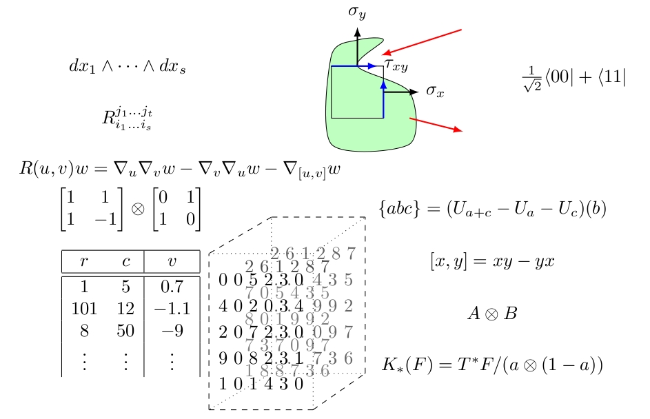
The scheme for defining tensors is thus to apply the rigorous axioms to a tensor space, then the actual objects we call tensors are free to take on diverse meanings. Indeed in the literature one finds tensors of row vectors, matrices, lists of matrices, arrays, functions, differential operators, integrals, multiplication tables, algebras, modules, multilinear maps, curvatures, stress formulas, quantum entanglements, meta-data, big data, statistics, and more. See the image above
Below we walk through all the ingredients but let us begin with the definition now even before we detail all the semantics so that the essential words and the arc of the narrative come into focus.
A tensor space is a vector space $T$ equipped with a linear representation \(\langle \cdot |:T\to V_0\oslash\cdots \oslash V_{\ell}\) into the space $V_0\oslash\cdots\oslash V_{\ell}$ of multilinear maps with reference frame $V_0,\ldots,V_{\ell}$. Tensors are elements of tensor spaces.
Therefore it must be emphasized that to be a tensor it is not enough to be a vector! Indeed, every tensor $t\in T$ demands also an interpretation as a multilinear map: \(\langle t|:V_{\ell}\times\cdots\times V_1\rightarrowtail V_0.\) (The symbol $\rightarrowtail$ signifies multilinear as we shall define below.) This is the real power in the study of tensors that turns grids of numbers and diverse objects into a system that can be studied cohesively as one theory.
Computing with tensors
If you are looking to use tensors in software take a look at Chapter 2 of our manual for our Magma software found here.
Notation with Dirac Bra-c-kets
We here define tensor spaces over vector spaces, but as anyone who knows the word “module” can guess, these definitions apply far more broadly.
Start with vector spaces $V_0$ and $V_1$, over any field $K$, the real numbers if you have no imagination or the $p$-adics if you are a hipster. A linear map $\langle f|:V_1\to V_0$ means as usual that \(\langle f|\alpha u+\beta v\rangle=\alpha \langle f|u\rangle +\beta \langle f|v\rangle.\)
For contextual brevity we let Greek fonts denote scalars and Roman fonts vectors. We include this well-known concept mostly as excuse to demonstrate our Dirac notation.
Functions on vectors $\langle f\mid$ are read “bra-f”, while vectors $\mid u\rangle$ are read “ket u”. These combine to make a “bra”c”ket” $\langle f\mid u\rangle$.
Yes, this notation is a gimmick but it is memorable and adopted heavily in physics. Having experimented with many alternative notations this notation appears the most light-weight for the calculus of tensors. One critical difference is that we here are content to map into any vector space $V_0$. In physics one assumes $V_0=K$, in fact, one assumes $K=\mathbb{C}$. We make no such conventions.
$\oslash$ and bilinear maps
The set fo linear maps we write as follows. \(V_0\oslash V_1 = \{ \langle f|:V_1\to V_0\} = \hom_K(V_1,V_0).\) Nothing is wrong with the use of $\hom$, except that it makes for extra-ordinarily long lines in what we do next. At the end we also pause to note some handy calculus that is suggested by the division-like notation $\oslash$.
Since $V_0\oslash V_1$ is comprised of linear maps then \(V_0\oslash V_1\oslash V_2 := (V_0\oslash V_1)\oslash V_2\\ = \{ \langle f|:V_2\to (V_1\to V_0)\}\) consists of bi-linear maps.
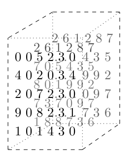
Bilinear is just the name so lets give it some content through an example. Recall that a linear map $\langle f|:K^b\to K^a$ can be given by a $(a\times b)$-matrix, each column being the image $\langle f|e_i\rangle$ of the $i$-th coordinate vector $e_i$ from the domain. Therefore $\langle f|: K^c\to (K^b\to K^a)$. \(\langle f|e_i\rangle\in \mathbb{M}_{a\times b}(K).\) So $\langle f|$ could be described from a list $[M_1,\ldots,M_c]$ of $(a\times b)$-matrices. Of course a matrix is a list of columns where we blur the edge between the columns, so $\langle f|$ can likewise be thought of as 3-dimensional grid of numbers.

Software packages are keen to take such creatures as the very definition of a tensor, but doing so ignores almost all applications. So these are just examples.
We could evaluate a bilinear map $\langle f|$ on $|v_2\rangle$ producing \(\langle f|v_2\rangle :V_1\to V_0\) But then why not evaluate on a pair of inputs as follows. \(\langle f|v_2,v_1\rangle :=\langle f|v_2\rangle |v_1\rangle\in V_0\) At this point we could just as well think of bilinear is a map on pairs: \(\langle f| : V_2\times V_1\rightarrowtail V_0\) The use of $\rightarrowtail$ makes it clear that $\langle f|$ is not to be confused with a linear map. Going back to list of matrices for a moment this could be defined as follows. \(\langle f|v_2,v_1\rangle = (v_2^{\top} M_1 v_1,\ldots,v_2^{\top} M_a v_1)\)
Indeed, \begin{align*} \langle f|\alpha u_2+\beta u_2’, u_1\rangle & = \alpha\langle f|u_2,u_1\rangle+\beta\langle f|u_2’,u_1\rangle\\ \langle f|u_2, \alpha u_1+\beta u_1’\rangle & = \alpha\langle f|u_2,u_1\rangle+\beta\langle f|u_2,u’_1\rangle \end{align*}
A lot of fuss is made about the scalars but in truth once we know $\langle f|$ is bilinear we can reconstruct the scalars for free through something called centroids. Trust us. So really you can ignore $\alpha$’s and $\beta$’s and focus on one key point:
Bilinear maps are distributive products.
To drive that point home write $u_2*u_1 := \langle f \mid u_2,u_1\rangle$ and let $\alpha=\beta=1$. Then all we have said is the following.
\begin{align*} (u_2+u’_2)*u_1 & = u_2*u_1 + u’_2*u_1\\ u_2*(u_1+u’_1) & = u_2*u_1 + u_2*u’_1 \end{align*}
Multilinear maps
Inducting further \(V_0\oslash V_1\oslash V_2\oslash V_3\) consists of tri-linear maps. Just as many linear maps can be captured by matrices (lists of vectors), and several bilinear maps by list of matrices, so too a trilinear map are often thought of as lists of bilinear maps. The process continues without end. The set \(V_0\oslash \cdots \oslash V_{\ell+1} := (V_0\oslash \cdots\oslash V_{\ell})\oslash V_{\ell+1}\) consists of multi-linear maps. Once more the scalars are barely important. You should think of these are large distributive products. Something like trinomials $xyz$, i.e.
\[\begin{aligned} (x+x')yz & = xyz+x'yz \\ x(y+y')z & = xyz+xy'z\\ xy(z+z') & = xyz+xyz'. \end{aligned}\]Our Dirac styled notation lets us capture these higher arity products. Here we have a trinary distributive product $\langle t|$:
\[\begin{aligned} \langle t| v_3+v'_3,v_2,v_1\rangle & = \langle t | v_3,v_2,v_1\rangle+\langle t|v'_3,v_2,v_1\rangle \\ \langle t| v_3,v_2+v'_2,v_1\rangle & = \langle t | v_3,v_2,v_1\rangle+\langle t|v_3,v'_2,v_1\rangle \\ \langle t| v_3,v_2,v_1+v'_1\rangle & = \langle t | v_3,v_2,v_1\rangle+\langle t|v_3,v_2,v'_1\rangle. \end{aligned}\]There is a little notational manuever to cut down on repetition. Since we bothered to index our variables, there is no need to put them in order. So distributive in all variables can be captured with one identity. \((\forall a)\quad \langle t|v_a+v'_a,v_{\bar{a}}\rangle=\langle t|v_a,v_{\bar{a}}\rangle+\langle t|v'_a,v_{\bar{a}}\rangle.\) Her $\bar{a}$ means the complement of the index $a$ in ${1,\ldots,\ell}$.
